Welcome to Jaehyek's Blog!

• eMMC & UFS FTL (3)

  2016-12-07

  Jaehyek

  eMMC-UFS

  eMMC  UFS  FTL

  FTL Functions

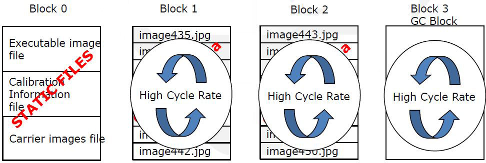
  Wear Leveling

  • Wear leveling software monitors Flash erase block cycling and guarantees that all erase block are cycled about the same number of times.
  • Some files are seldom changed, while others may be changed frequently. If all files were updated at the same frequency, wear leveling would not be necessary.

  Handling Device Error

  • Handing Bad Block for NAND
  • NAND permits 1-2% factory or run time bad blocks
  • BD tract this information through marking to the head of block or separate table

  • BD have to have strategy to decide run-time bad block when read/write/erase error happens

  • Handling Bit error for NAND
  • One or a few bit error happens rarely in NAND.
  • Error collection code can allow the area to live instead of throw it away by marking Bad block

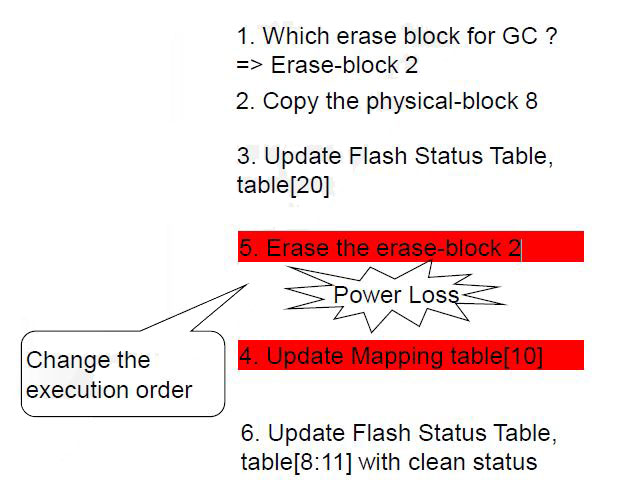
  Power Loss Problem

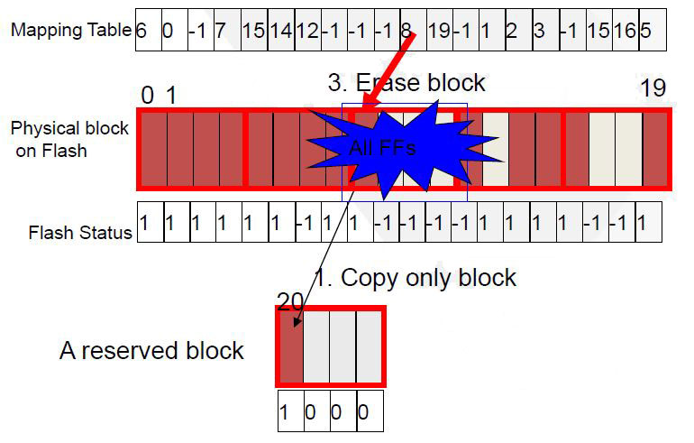
  • Power loss break BD’s integrity in various way
  • Crash BD and make BD be disable to mount

  • Point wrong physical block for a virtual sector

  • Lost Data Case

  

  Read All

  ---

• eMMC & UFS FTL (2)

  2016-12-07

  Jaehyek

  eMMC-UFS

  eMMC  UFS  FTL

  GC & Write Amplification

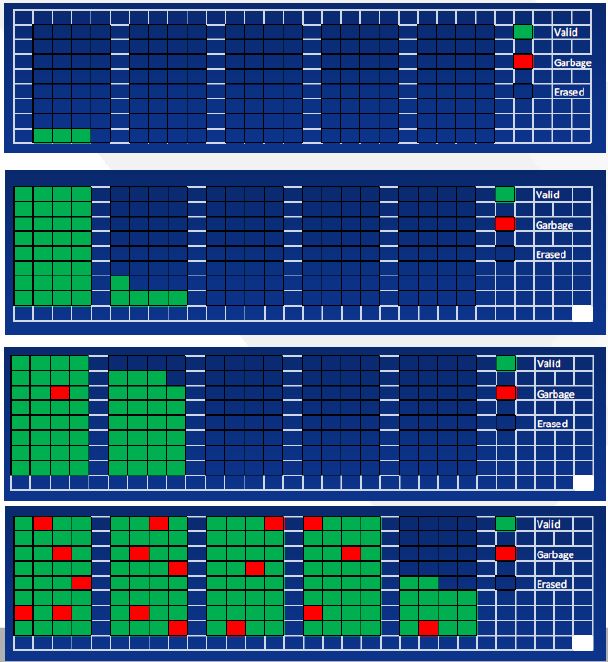
  Garbage collection

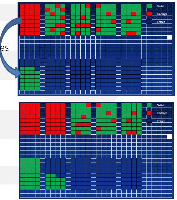
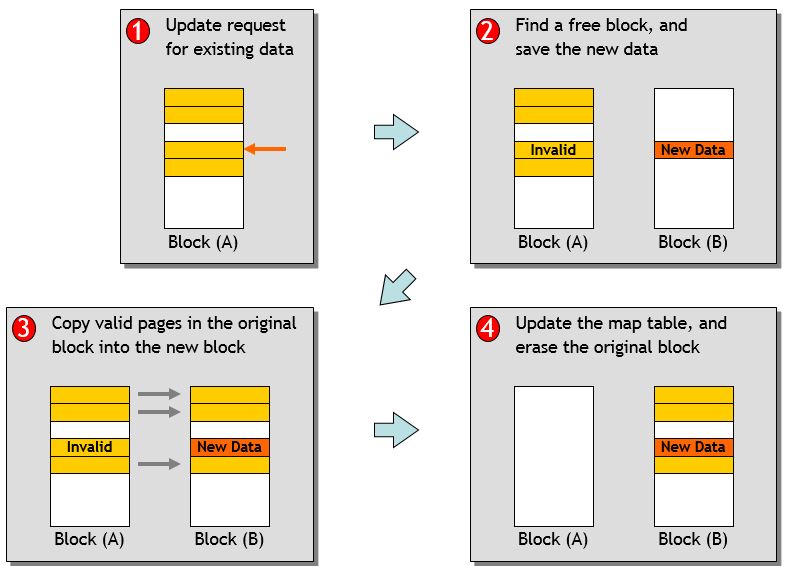
  • FTL fills incoming data into the erased nand-block

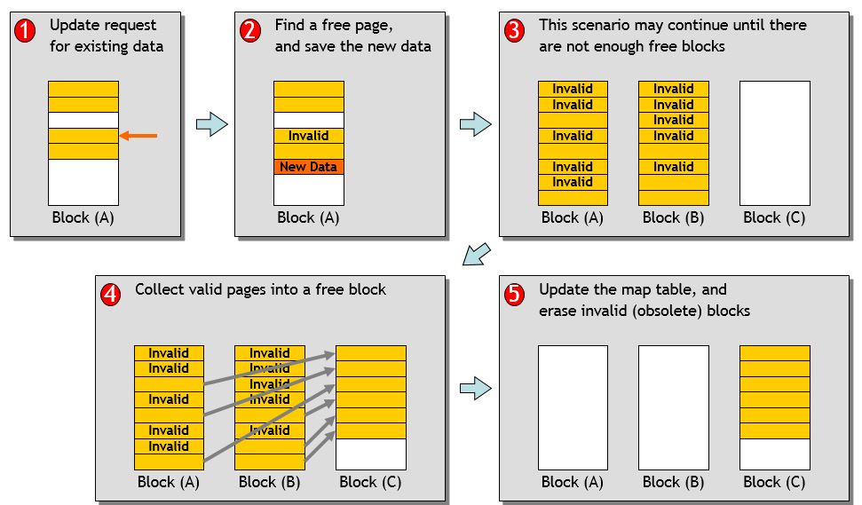
  • Overwriting the same logical block goes to new erase nand block ( copy on write)

  • No free space => Do GC

  • Copy valid pages

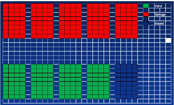
  • Copy done !!

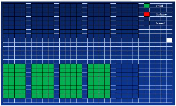
  • Erase 5 blocks, GC done

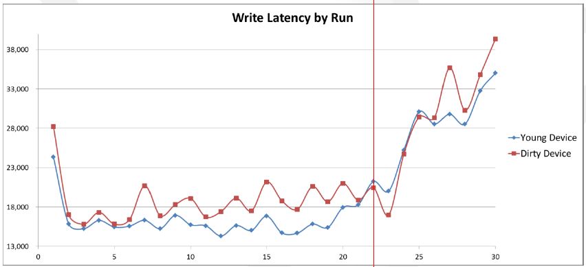
  • Performance degradation by GC

  Write amplification

  • Write amplification = ( Data written to the flash memory) / ( Data written by host )
  • WA KEY = Garbage collection Map(FTL-meta) update Wear-leveling
  Read All

  ---

• eMMC & UFS FTL (1)

  2016-12-07

  Jaehyek

  eMMC-UFS

  eMMC  UFS  FTL

  FTL (Flash Translation Layer)

  Flash’s Limitation

  • No overwrite without Erase
  • Big erase block : ex. 2MB
  • Factory Bad Block and Run time Bad Block
  • Run time bit error
  • Limited Lifetime : ex) Erase 5K for an Erase Block

  FTL’s Roles

  • Flash Translation Layer : mapping virtual sector to physical block
  • Garbage Collection
  • Power Loss Recovery
  • Error Correction
  • Bad Block Management
  • Wear leveling

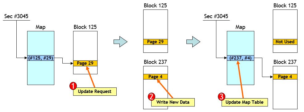
  Address Remapping

  • Address mapping table
  • Trying to update data of (Sector #3045) stored NAND(Block #125, Page #29)

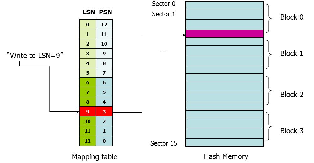
  Sector Mapping

  LSN: Logical Sector Number PSN : Physical Sector Number

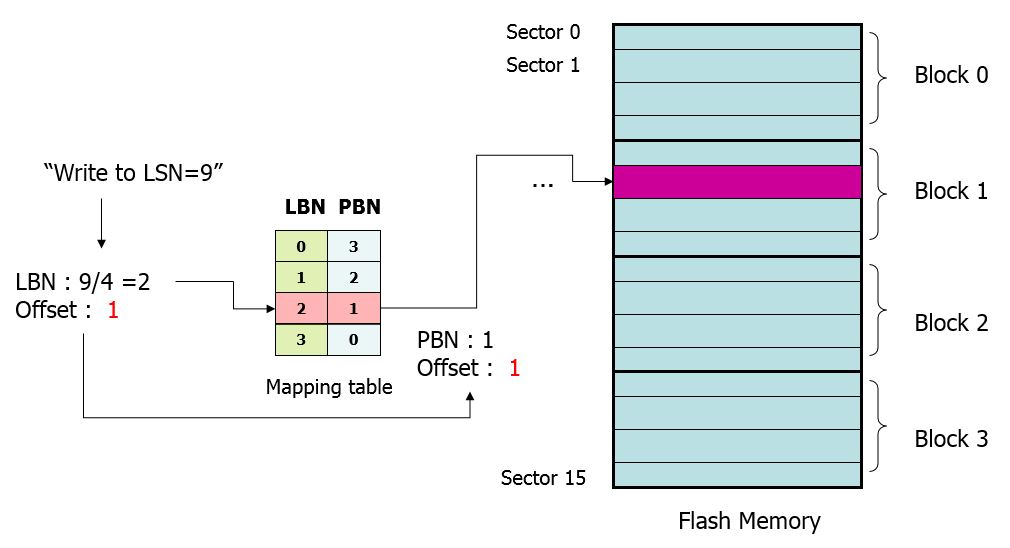
  Block Mapping

  LBN: Logical Block Number PBN : Physical Block Number

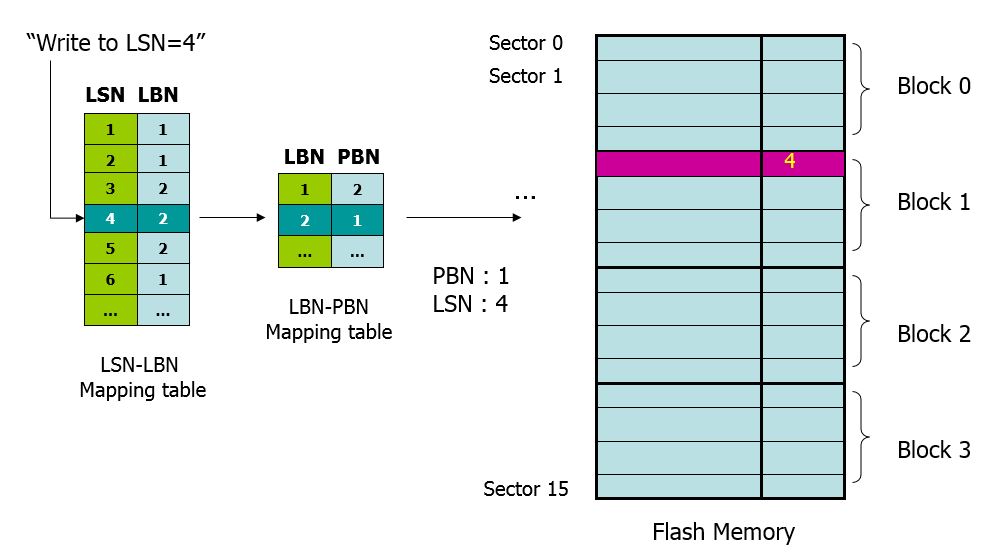
  Hybrid Mapping

  

  Merge

  

  Garbage Collection

  

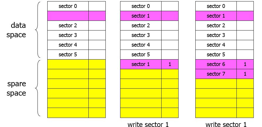
  Spare Space method

  • Mitsubishi
  • Data space : in-place
  • Spare space : out-of-place

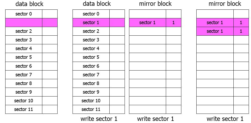
  Mirror Block method

  • M-Systems (FMAX)

  Log Block method

  • SNU
  • write (5,1) (5,1) (5,2) (5,4) (5,4) (5,1)
  • write (6,3) (8,0) (8,1) (8,2) (8,3) (8,4) (8,5)

  Full Associative Sector Translation : FAST

  

  • write (5,1) (5, 1) (6. 2) (6, 4) (8, 4) (5, 1), (8, 3)
  Read All

  ---

• Health Information Sites

  2016-12-07

  Jaehyek

  Health

  Health  Information  Sites

  건강 정보 sites

  • ‘암세포’ 자살시키는 식품 15가지
  Read All

  ---

• Causes of learning slowdown phenomenon

  2016-12-07

  Jaehyek

  Deep-Learning

  Deep-Learning  Machine-Learning  slowdown

  refer to http://laonple.blog.me/220548474619

  Problem of Neural Network Learning Speed - Learning Slowdown

  If the difference between the original value (the result of the training data) and the actual value of network is large, Will the learning really work ?
  Generally the method of MSE ( Mean Square Error ) to use the cost function of neural network doesn’t work well unfontunately ‘

  Why?
  in case that you use the cost function as MSE and Sigmoid as active function, it is because that a problem is assoicated with Sigmoid characteristics

  Cause of learning slowdown of neural network – due to the differential nature of sigmoid function
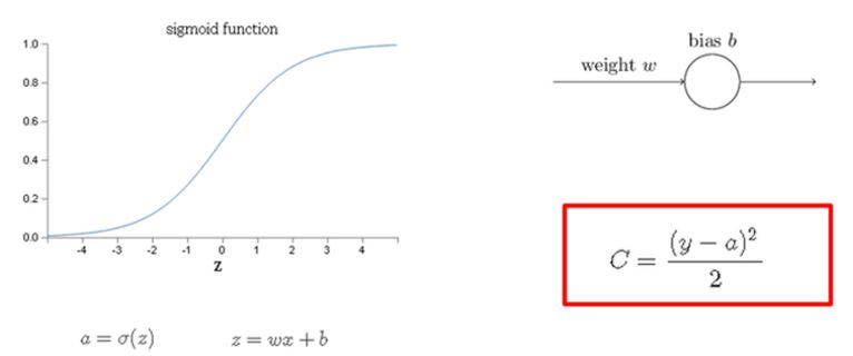
  To explain easily let’s guess that we have one neuron, w weight, b bias and active function as sigmoid like as the below picture
  

  When a input is x, the input of neuron is z = wx + b
  passing the active function σ(z), the output a comes out.

  

  if the output is y when a input is x ,
  the cost function is the red box like as above picture.

  Here (y – a) is error , and make the error back-propagate. and then
  The larger the error , the faster the learning should be.

  As we inspected with back-propagation page,
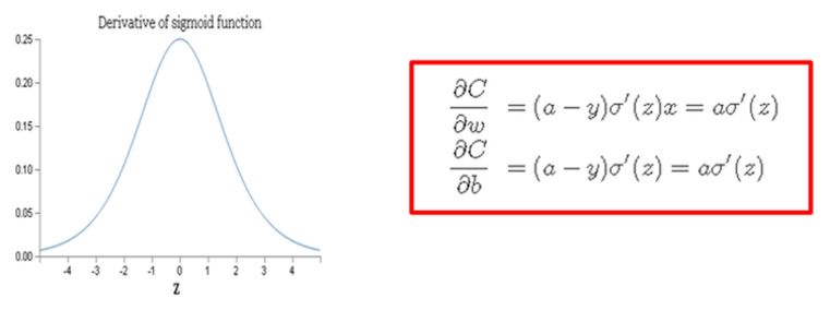
  To update the value of weight and bias the cost function C performs partial-differential for weight and bias. After performing the partial-differential, the result as the below red box comes out.

  

  As you can see from the above equation,
  the partial differential value of weight and bias have the multiplication with sigmoid derivative.
  Right this is a main curprit.

  When we have the derivative for sigmoid function, the result like as the above picture comes out.
  That is, z equal to 0 , then get the maximum, and the farther from 0, the smaller to 0 the derivative value goes.
  That is, the updated value of weight and bias has a form to multiply the very small value,
  and then although (a-y) item is very large, finally the z value would become a very small value, and make the learning speed slowdown.

  Cause of learning slowdown of neural network – due to the gradient decent nature
  

  When we see the partial differential equation of C/W,
  the value of (a - y ) becomes small, that is, the target value and the real value of network become almost same ,
  the value of (a - y ) becomes again close to 0, and finally the updated value of weight and bias become smaller.
  finally when goes close to 0, and the learning speed become slowdown.

  This is due to the structural characteristics of the gradient descent method.
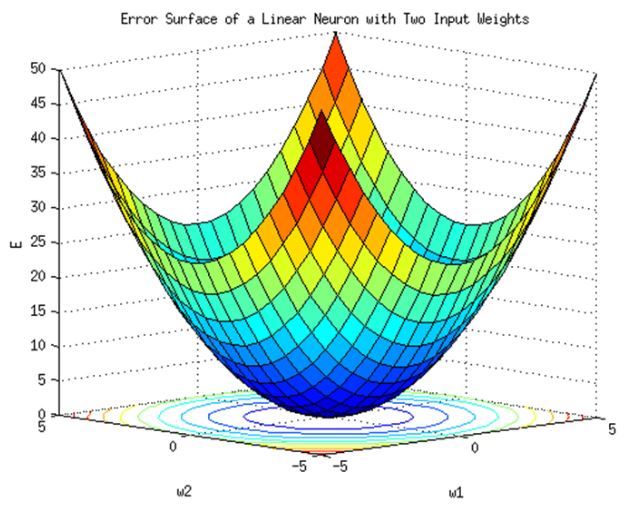
  As we saw earlier in “class 8”, the gradient descent method is the result.

  

  When you drop the ball from a high place,
  No matter where you start,
  The larger the gradient (the larger the gradient), the faster it moves.
  Then when it comes to the bottom (ie near the target)
  Because there is little slope, the speed at which the ball rolls is slowed down.

  Finally when (a - y ) goes close to 0, the learning speed become slow,
  a phenomenon occurs in which the result of learning does not improve so much even if the learning is further performed.

  Cross-Entropy The cross-entropy cost function is defined as follows.
  Where y is the expected value,
  Assuming that a is a value output from the actual network,
  Let n be the number of training data.

  

  Using the sigmoid function as an active function

  

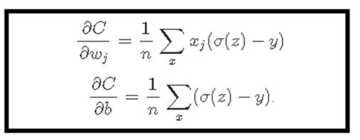
  As we initially expected, we were able to get results that were proportional to the difference between expected and actual output.
  As a result, when the learning is performed using the CE cost function,
  Because learning progresses much faster
  Nowadays, we use CE cost function more than MSE

  Read All

  ---

• Avoid Overfitting

  2016-12-07

  Jaehyek

  Deep-Learning

  Deep-Learning  Machine-Learning  overfitting

  refer to http://laonple.blog.me/220522735677

  What is the overfitting ?

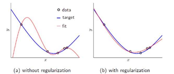
  Let’s look over the above picture. Given some blue points, guess a curve to represent the points

  • picture(a) : seems like that a simple line has a error to represent those.
  • picture(c) : is inferenced that the lime represent the whole points perfectly. but Although it got the optimization results, if given a point, that would produce the wrong result. we call this overfitting !!!.
  • picture(b) : the line represents the whole points although it has a little error. also if given a point , it would still represent the whole thing well.

  How to resolve the overfitting ?

  The perfect solution to avoid the overfitting is to collect a lot of data. But it would make a lot of time or cost. sometime it would be difficult or impossible to gathering more data.

  Additinally if given a lot of training data, increasing training time would also become a issue.

  When statistical inferencing or running the machime learning normally, the cost function or error function goes to a lower error. But just simple lower error can go to bad result.

  Solution 1 ) the below picture showes that the regularization makes good results.

  

  * the mathematical presentation of Regularization .

  

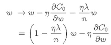
  C0 = Cost function n = data count λ = traning rate w = weights

  the learning direction is to go the lower cost , and also the w value got to go to lower

  By Differentiating with w , finally a new w get to become like below .

  

  At the above, (1 – ηλ/n)w will make the w value lower as the n increases.
  This is called “weight decay”.

  Solution 2 ) Intelligent training data generation using Affine Transform

  

  The above figure shows data obtained by rotating the left-handed data counter-clockwise by 15 degrees.
  After this affine transform,Various data can be obtained.
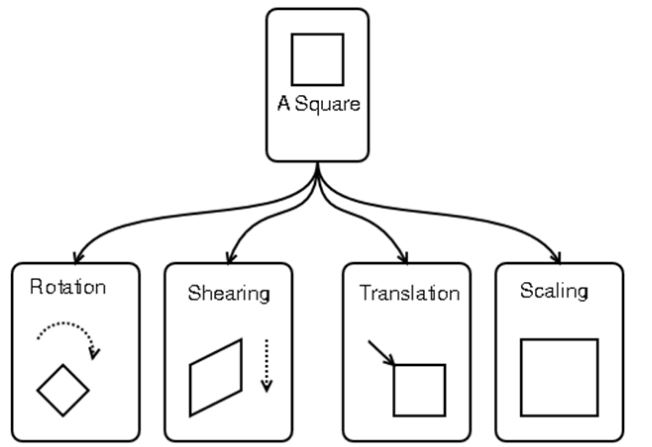
  Affine transform has four operations as shown below, Combining these can provide a lot of training data
  

  

  Solution 3 ) Intelligent training data generation using Elastic Distortion

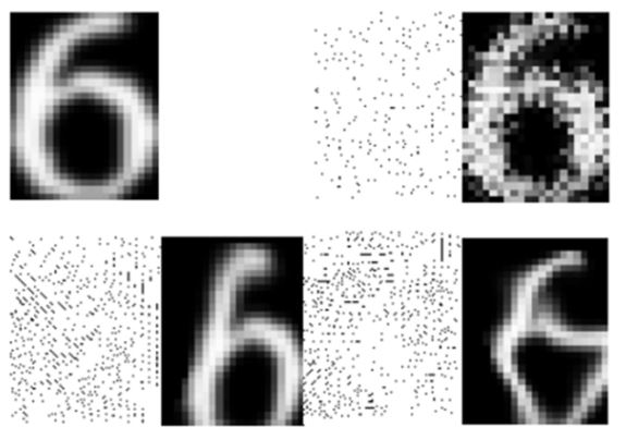
  Create a displacement vector in various directions as shown below.
  This allows us to create more complex forms of training data, It will be obvious that this will be a training data set useful for handwriting recognition

  

  In the case of speech recognition, similar training data can be generated.
  For example, after recording with no noise, Through synthesis with various background noise,
  Various training data sets can be created.

  Solution 4) Dropout

  ** Advantage and Disadvantage of increasing number of Hiddern Layers.**
  In general, as the number of hidden layers increases in neural network,
  In other words, a deep neural network can improve the ability to solve more problems

  However, as the net size increases, the possibility of overfitting increases,
  and there is a problem that the learning time for the neural network is lengthened,
  the amount of learning data should be increased too to get a proper results .

  Dropout overview
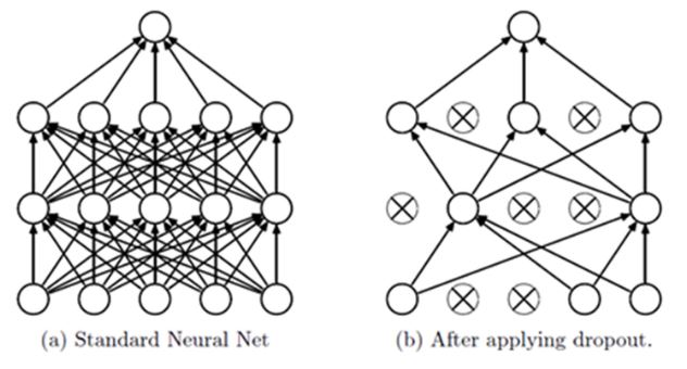
  As the network size increase like this, the method to avoid the overfitting is dropout,
  it has not been more than 10 years since the paper was published.

  Dropout, when learning about figure (a) below,
  Instead of learning about all the layers in the network
  As shown in (b), some neurons in the input layer or hidden layer in the network are dropped out
  The learning is performed through the reduced neural network.
  If you finish learning the omitted network during a certain mini-batch period,
  Repeated learning is performed while dropping out other neurons randomly

  

  Dropout effect
  

  ① Voting
  The first reason for dropout is because of the voting effect.
  If you are learning using a reduced network during a certain mini-batch period,
  The network is overfitting itself,
  If you learn about other networks during other mini-batch intervals,
  The network is again overfitting to some extent.
  

  When this process is repeated randomly,
  Since the average effect by voting can be obtained,
  As a result, you can get a similar effect to regularization
  

  ② Effect to avoid Co-adaptation
  Another reason is the avoidance of co-adaptation.

  As we have seen in Regularization,
  When the bias or weight of a particular neuron has a large value
  As its influence increases, the learning rate of other neurons slows
  There are cases where learning does not work properly.

  But when you do the dropout,
  As a result, the weight or bias of any neuron is not affected by a particular neuron
  As a result, neurons can avoid co-adaptation.
  

  It is possible to construct a more robust network that is not affected by specific learning data or data.

  This means that life forms that exist on Earth for a long time
  Binding genes through positive reproduction, not gene replication
  Just as stronger genes survive the selection of nature
  

  Read All

  ---