Canadian Institute for Advanced Research (CIFAR)
Google DeepMind’s Deep Q-learning playing Atari Breakout
Multinomial classification
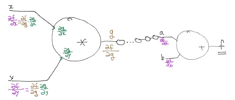
Back propagation
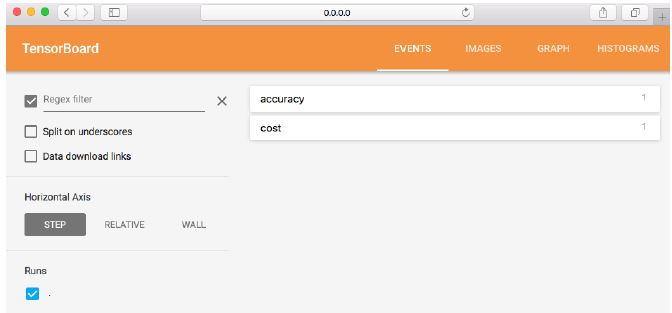
5 steps of using tensorboard
- From TF graph, decide which node you want to annotate
- with tf.name_scope(“test”) as scope:
- tf.histogram_summary(“weights”, W), tf.scalar_summary(“accuracy”, accuracy)
- Merge all summaries
- merged = tf.merge_all_summaries()
- Create writer
- writer = tf.train.SummaryWriter(“/tmp/mnist_logs”, sess.graph_def)
- Run summary merge and add_summary
- summary = sess.run(merged, …); writer.add_summary(summary);
- Launch Tensorboard
- tensorboard –logdir=/tmp/mnist_logs
- You can navigate to http://0.0.0.0:6006
import tensorflow as tf
import numpy as np

xy = np.loadtxt('07train.txt', unpack=True)
x_data = np.transpose(xy[0:-1])
y_data = np.reshape(xy[-1], (4, 1))

print x_data
print y_data

X = tf.placeholder(tf.float32, name='x-input')
Y = tf.placeholder(tf.float32, name='y-input')

w1 = tf.Variable(tf.random_uniform([2, 5], -1.0, 1.0), name='weight1')
w2 = tf.Variable(tf.random_uniform([5, 10], -1.0, 1.0), name='weight2')
w3 = tf.Variable(tf.random_uniform([10, 10], -1.0, 1.0), name='weight3')
w4 = tf.Variable(tf.random_uniform([10, 10], -1.0, 1.0), name='weight4')
w5 = tf.Variable(tf.random_uniform([10, 10], -1.0, 1.0), name='weight5')
w6 = tf.Variable(tf.random_uniform([10, 10], -1.0, 1.0), name='weight6')
w7 = tf.Variable(tf.random_uniform([10, 10], -1.0, 1.0), name='weight7')
w8 = tf.Variable(tf.random_uniform([10, 1], -1.0, 1.0), name='weight8')

b1 = tf.Variable(tf.zeros([5]), name="Bias1")
b3 = tf.Variable(tf.zeros([10]), name="Bias3")
b2 = tf.Variable(tf.zeros([10]), name="Bias2")
b4 = tf.Variable(tf.zeros([10]), name="Bias4")
b5 = tf.Variable(tf.zeros([10]), name="Bias5")
b6 = tf.Variable(tf.zeros([10]), name="Bias6")
b7 = tf.Variable(tf.zeros([10]), name="Bias7")
b8 = tf.Variable(tf.zeros([1]), name="Bias8")

L2 = tf.nn.relu(tf.matmul(X, w1) + b1)
L3 = tf.nn.relu(tf.matmul(L2, w2) + b2)
L4 = tf.nn.relu(tf.matmul(L3, w3) + b3)
L5 = tf.nn.relu(tf.matmul(L4, w4) + b4)
L6 = tf.nn.relu(tf.matmul(L5, w5) + b5)
L7 = tf.nn.relu(tf.matmul(L6, w6) + b6)
L8 = tf.nn.relu(tf.matmul(L7, w7) + b7)

hypothesis = tf.sigmoid(tf.matmul(L8, w8) + b8)

with tf.name_scope('cost') as scope:
    cost = -tf.reduce_mean(Y * tf.log(hypothesis) + (1-Y) * tf.log(1 - hypothesis))
    cost_summ = tf.summary.scalar("cost", cost)

with tf.name_scope('train') as scope:
    a = tf.Variable(0.1)
    optimizer = tf.train.GradientDescentOptimizer(a)
    train = optimizer.minimize(cost)

w1_hist = tf.summary.histogram("weights1", w1)
w2_hist = tf.summary.histogram("weights2", w2)

b1_hist = tf.summary.histogram("biases1", b1)
b2_hist = tf.summary.histogram("biases2", b2)

y_hist = tf.summary.histogram("y", Y)

init = tf.global_variables_initializer()

with tf.Session() as sess:
    sess.run(init)

    merged = tf.summary.merge_all()
    writer = tf.summary.FileWriter("./logs/xor_logs", sess.graph)

    for step in xrange(20000):
        sess.run(train, feed_dict={X: x_data, Y: y_data})
        if step % 200 == 0:
            summary = sess.run(merged, feed_dict={X: x_data, Y: y_data})
            writer.add_summary(summary, step)
            print step, sess.run(cost, feed_dict={X: x_data, Y: y_data}), sess.run(w1), sess.run(w2)

    correct_prediction = tf.equal(tf.floor(hypothesis+0.5), Y)

    accuracy = tf.reduce_mean(tf.cast(correct_prediction, "float"))
    print sess.run([hypothesis, tf.floor(hypothesis+0.5), correct_prediction], feed_dict={X: x_data, Y: y_data})
    print "accuracy", accuracy.eval({X: x_data, Y: y_data})
ReLU: Rectified Linear Unit
- L1 = tf.sigmoid(tf.matmul(X, W1) + b1)
-
L1 = tf.nn.relu(tf.matmul(X, W1) + b1)
- maxout = max(w1x + b1, w2x + b2 )
Activation functions on CIFAR-10
Need to set the initial weight values wisely
- Not all 0’s
- Challenging issue
- Hinton et al. (2006) “A Fast Learning Algorithm for Deep Belief Nets”
- Restricted Boatman Machine (RBM) : not used these day
- recreate input ( encoder/decoder )
- Deep Belief Net ( initialized by RBM )
Good news
- No need to use complicated RBM for weight initializations
- Simple methods are OK
- Xavier initialization
- He’s initialization
- Makes sure the weights are ‘just right’, not too small, not too big
- Using number of input (fan_in) and output (fan_out)
# Xavier initialization
# Glorot et al.2010
W = np.random.randn(fan_in, fan_out)/np.sqrt(fan_in)

# He et al.2015
W = np.random.randn(fan_in, fan_out)/np.sqrt(fan_in/2)
- prettytensor implementation
def xavier_init(n_inputs, n_outputs, uniform=True):
  """Set the parameter initialization using the method described.
  This method is designed to keep the scale of the gradients roughly the same
  in all layers.
  Xavier Glorot and Yoshua Bengio (2010):
           Understanding the difficulty of training deep feedforward neural
           networks. International conference on artificial intelligence and
           statistics.
  Args:
    n_inputs: The number of input nodes into each output.
    n_outputs: The number of output nodes for each input.
    uniform: If true use a uniform distribution, otherwise use a normal.
  Returns:
    An initializer.
  """
  if uniform:
    # 6 was used in the paper.
    init_range = math.sqrt(6.0 / (n_inputs + n_outputs))
    return tf.random_uniform_initializer(-init_range, init_range)
  else:
    # 3 gives us approximately the same limits as above since this repicks
    # values greater than 2 standard deviations from the mean.
    stddev = math.sqrt(3.0 / (n_inputs + n_outputs))
    return tf.truncated_normal_initializer(stddev=stddev)
- Activation functions and initialization on CIFAR-10
- Geoffrey Hinton’s summary of findings up to today
- Our labeled datasets were thousands of times too small.
- Our computers were millions of times too slow
- We initialized the weights in a stupid way
- We used the wrong type of non-linearity
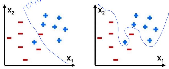
Overfitting
- Solutions for overfitting
- More training data
- Reduce the number of features
- Regularization
- Let’s not have too big numbers in the weight
- Let’s not have too big numbers in the weight
-
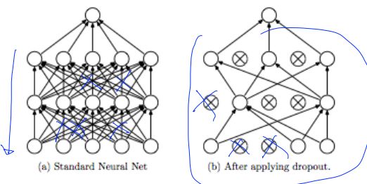
Dropout: A Simple Way to Prevent Neural Networks from Overfitting [Srivastava et al. 2014]
-
Regularization: Dropout “randomly set some neurons to zero in the forward pass”
- dropout TensorFlow implementation
dropout_rate = tf.placeholder("float") _L1 = tf.nn.relu(tf.add(tf.matmul(X, W1), B1)) L1 = tf.nn.dropout(_L1, dropout_rate)- TRAIN:
sess.run(optimizer, feed_dict={X: batch_xs, Y: batch_ys, dropout_rate: 0.7})
- EVALUATION:
print "Accuracy:", accuracy.eval({X: mnist.test.images, Y:mnist.test.labels, dropout_rate: 1})


